Basics of electronic ...

The purpose of this topic is to learn about the properties and parameters of operational amplifiers and methods of measuring the parameters and characteristics of operational amplifiers.

The operational amplifier will be presented first as an ideal element, and then as a real one.

The ideal operational amplifier is an electronic circuit with the following three main characteristics:

1) the characteristics of the amplifier are as shown in Fig.1,

2) the input resistance is infinite (the input is as opening),

3) the output resistance is equal to zero (the amplifier behaves at the output as an ideal voltage source).

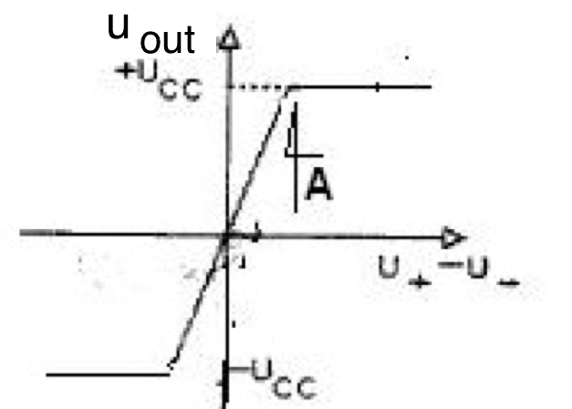
Figure 1

The course of the characteristics in Fig. 1 shows that generally the operational amplifier is a non-linear element and only for small signals it is a linear element, i.e. its output voltage is proportional to the input voltage. In this linear range of the characteristics, the operational amplifier behaves as a voltage-controlled voltage source (see Fig. 3), with the characteristic parameter of the amplifier being the slope of the linear part of the characteristic A - the gain of the operational amplifier with an open feedback loop (the need to use a long name results from the need to distinguish A from the voltage gain \(k_u\) of an amplifier built using an operational amplifier and covered by a negative feedback loop - see below).

The symbol of the amplifier presented in Fig. 2a contains the outputs used to supply the DC energy necessary for its operation (marked \(+U_{CC}\) and \(–U_{CC}\)) and the outputs of the amplified signals \(U_{+ } – U_{–}\) and amplified \(U_{out}\). 

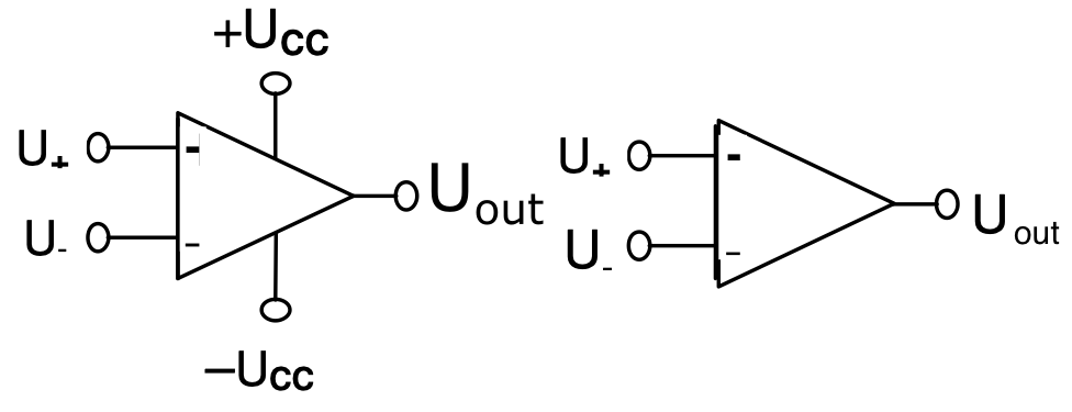
Figure 2

Bearing in mind the need for power supply, when considering the operation of signals, we often use the simplified diagram in Fig. 2b, which omit the power supply leads. All voltages are relative to ground, not shown here, and can be either positive or negative. The "+" and "-" subscripts refer to the non-inverting and inverting amplifier inputs, respectively. The input signal of the amplifier is the difference of these voltages \(U_{+} - U_{-}\). The equivalent diagram of the operational amplifier operating in the linear range, useful in the analysis of electronic circuits, is shown in Fig. 3. Recall that the non-inverting input acts on a sinusoidal signal or a DC voltage applied to it in such a way that the output voltage \(U_{out}\) will have the same phase or polarity as the voltage \(U_{+}\) , and in the case of an inverting input, the phase or polarity of the voltage changes to the opposite one.

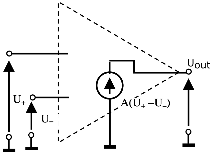
Figure 3

In linear applications, systems with feedback are used. One of the two most important systems of this type is the inverting amplifier shown in Fig. 4a, the other is the non-inverting amplifier shown in Fig. 4b.

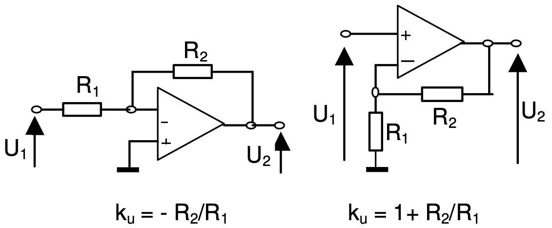
Figure 4

In both cases, a part of the signal is taken from the output and fed to the inverting input. Therefore, the feedback is negative and it reduces the gain of the whole system \(k_u\) compared to \(A\). It can be shown (see the formula for \(k_u\) at the end of the instruction) that if \(A\) is much greater than the quotient \(R_2/R_1\), then the gain \(k_u\) does not, to a very good approximation, depend on from \(A\), and thus from destabilizing factors such as temperature, dispersion of \(A\) values or changes in supply voltage \(U_{CC}\).

The transfer characteristic of a real operational amplifier (Fig. 5) is shifted relative to the characteristic of a balanced amplifier with finite gain.

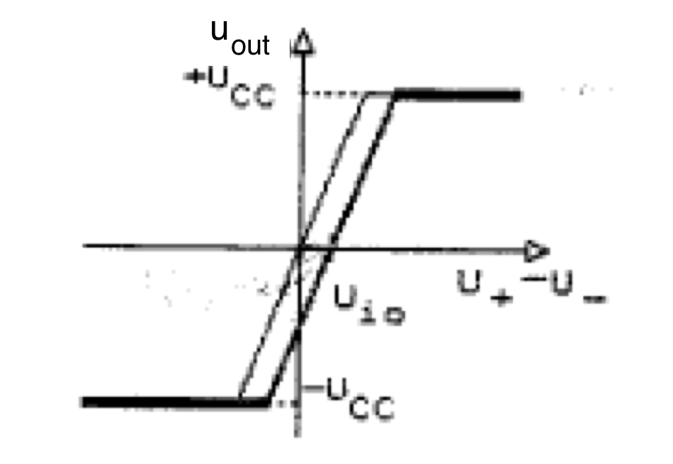
Figure 5

This shift is characterized by the input offset voltage \(U_{io}\), which can also be interpreted as the value of the DC voltage that must be applied to the input of the operational amplifier so that the DC voltage at the output of the operational amplifier is equal to zero.

In the equivalent diagrams of a real operational amplifier, the input offset voltage is represented by a voltage source with an electromotive force equal to \(U_{io}\) placed in series in the input circuit of the amplifier (Fig. 6).

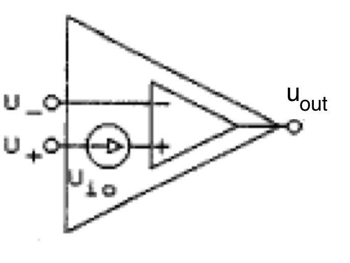
Figure 6

Since the offset voltage is small, on the order of a millivolt, it could be determined from the offset voltage measured at the output by dividing the measurement by the gain \(A\) of an open-loop op-amp, provided that the output of the op-amp is not saturation state. This condition is usually not met. In addition, the accuracy of the measurement would depend on the accuracy of the determination of the gain \(A\), which is usually not very high. Therefore, in practice, the offset voltage is measured when the operational amplifier operates in the inverting amplifier system (Fig. 7) with its input shorted, i.e. after the resistor \(R_1\) is shorted to ground.

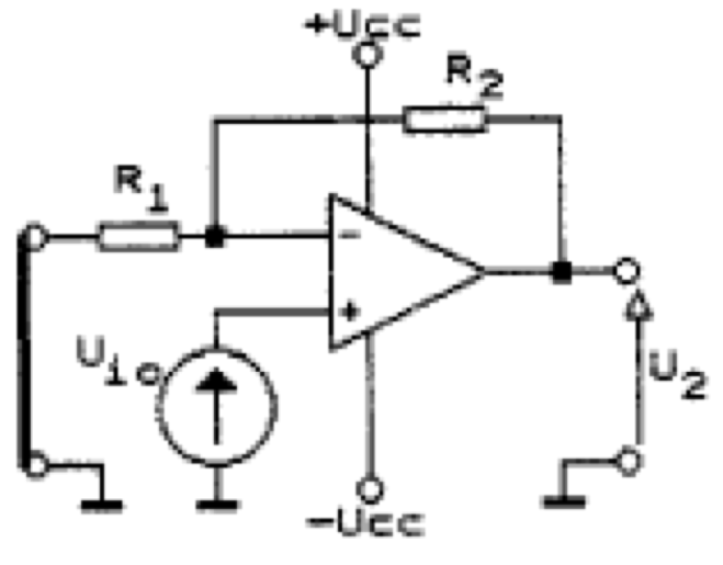
Figure 7

Then the output voltage is:

\( U_2 = -U_{io} \left ( 1 + \frac{R_2}{R_1} \right ) \)

Thus, by measuring \(U_2\) and knowing the ratio \(R_2/R_1\) (e.g. equal to 1000), you can determine the input offset voltage \(U_{io}\). The presented method does not take into account the influence of the input bias current \(I_{B}\) of the operational amplifier on the measurement result, because this influence can be compensated by the resistor \(R_3\), connected as shown in Fig. 8, with a resistance equal to the resistance resultant of the parallel connection \(R_2\) and \(R_1\).

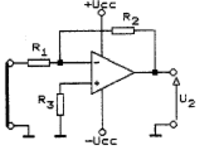
Figure 8

After compensating the influence of the input bias current \(I_B = (I_P + I_N)/2\), the influence of the input offset current \(I_{io} = I_P - I_N\) will remain, where \(I_P\) , \(I_N\) are the input bias currents of the non-inverting input ( \(I_P\) ) and the inverting input ( \(I_N\) ) respectively. The influence of the input offset current \(I_{io}\) can be neglected if the condition \(R_1I_{io} << U_{io}\) is met; therefore, in the measurement system shown in Fig. 8, it is desirable to use small resistances \(R_1\) and \(R_3\).

In many types of operational amplifiers, e.g. in the popular 741 type amplifier, the possibility of compensating the influence of the input offset voltage is provided. It consists in reducing the output voltage of the amplifier \(U_2\) to zero in the absence of a signal, i.e. when \(R_1\) is shorted to ground (Fig.9); an external multi-turn 10 kΩ potentiometer connected to pins 1, 5 and 4 is used for this purpose. Errors and problems in operational amplifier applications are caused not so much by the offset voltage, which can be compensated, as by its drifts, especially thermal ones.

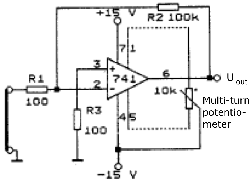
Figure 9