Operational amplifier and its parameters - theoretical introduction
Introduction (part 2)
In real operational amplifiers, the input bias currents \(I_P\) , \(I_N\) are different from zero.
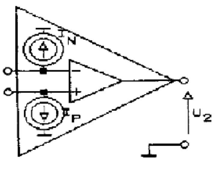
Figure 10
Fig. 10 shows the equivalent diagram of a real operational amplifier, considering only the input bias currents. They can be measured in the system shown in Fig. 11.
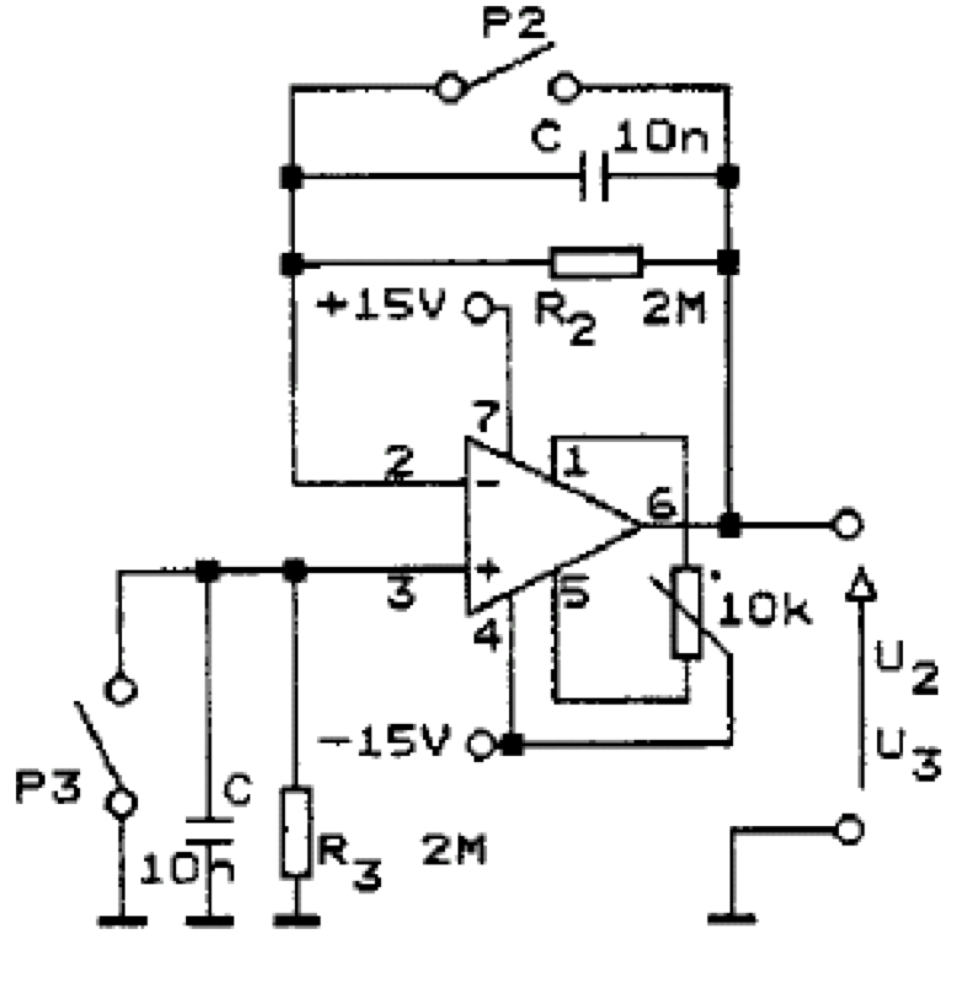
Figure 11
With the P3 switch closed and P2 open, the voltage \(U_2 = +R_2 I_N\) is measured at the output, from which the value of the current \(I_N\) can be determined.
Similarly, when the P2 switch is closed and P3 is open, there is a voltage \(U_3 = -R_3 I_P\) at the output, which allows to determine the value of the current \(I_P\).
The input bias current \(I_B\) is defined as the arithmetic mean of the \(I_P\) and \(I_N\) currents:
\(I_B =(I_P +I_N )/2 \)
The difference between these currents is the input offset current:
\(I_{io} = I_P − I_N \)
Determination of the input offset current on the basis of the previously determined \(I_P\) and \(I_N\) currents is burdened with a large error, because in practice these currents differ slightly from each other. Therefore, the input offset current \(I_{io}\) is determined in the circuit shown in Fig. 11 with both P2 and P3 circuit breakers open, measuring the output voltage \(U_1 = −RI_{io}\) , where \(R_2 = R_3 = R\), from which the current \(I_{io}\) can be determined, knowing the value \(R\) and measuring the voltage \(U_1\).
Measurements of other operational amplifier parameters, such as open-loop gain \(A\), differential input impedance \(R_d\) and common mode resistance \(R_c\), output resistance \(R_o\) and common mode rejection ratio CMRR are performed less often and usually with alternating current with frequencies of several Hertz (e.g. 5 Hz). Voltage measurement is then quite cumbersome and therefore an oscilloscope with DC input is usually used as a voltmeter. Resistance can be measured by the already known method of substituting a resistor in the input or output circuit, after such selection of its resistance that the output voltage drops to half the value occurring in the absence of a suitable resistor.The full equivalent circuit diagram of a real operational amplifier (without taking into account the noise properties) is shown in Fig. 12.
Frequently, the frequency response of an operational amplifier has the form shown in Fig. 13 (approximation with asymptotic characteristics, the gain on the ordinate axis is expressed in decibels, the frequency scale is logarithmic). It is described in the domain of the complex variable jω by the single pole function A(jω):
\( A (j \omega ) = \frac{A}{1+j \frac{\omega}{\omega_g}} \)
where the modulus for \( \omega << \omega_g \) does not depend on frequency, and for \( \omega >> \omega_g \) it decreases at a rate of -20 dB per decade. If the amplifier works in a phase inverting circuit with resistors \(R_1\) and \(R_2\), then its gain, taking into account the gain \(A\) of the open-loop operational amplifier, is:
\( ku = - \frac{R_2}{R_1} \frac{A}{A+1+\frac{R_2}{R_1}} \)
and the modulus \(|k_u(j\omega )|\) is a similar function of frequency as the modulus |A(jω)| (fig.13). It can be said that the bandwidth of feedback amplifiers increases because the so-called the gain bandwidth product, i.e. the product of the gain modulus in the flat part of the characteristic and the bandwidth for a 3 dB drop, is a constant value: \(|k_u|B = const\) . This theorem only holds for single pole functions. The frequency at which the gain module reaches 0 dB is denoted as \(f_T\) and is one of the dynamic parameters of the op-amp (equal gain area in the case of a single pole function).
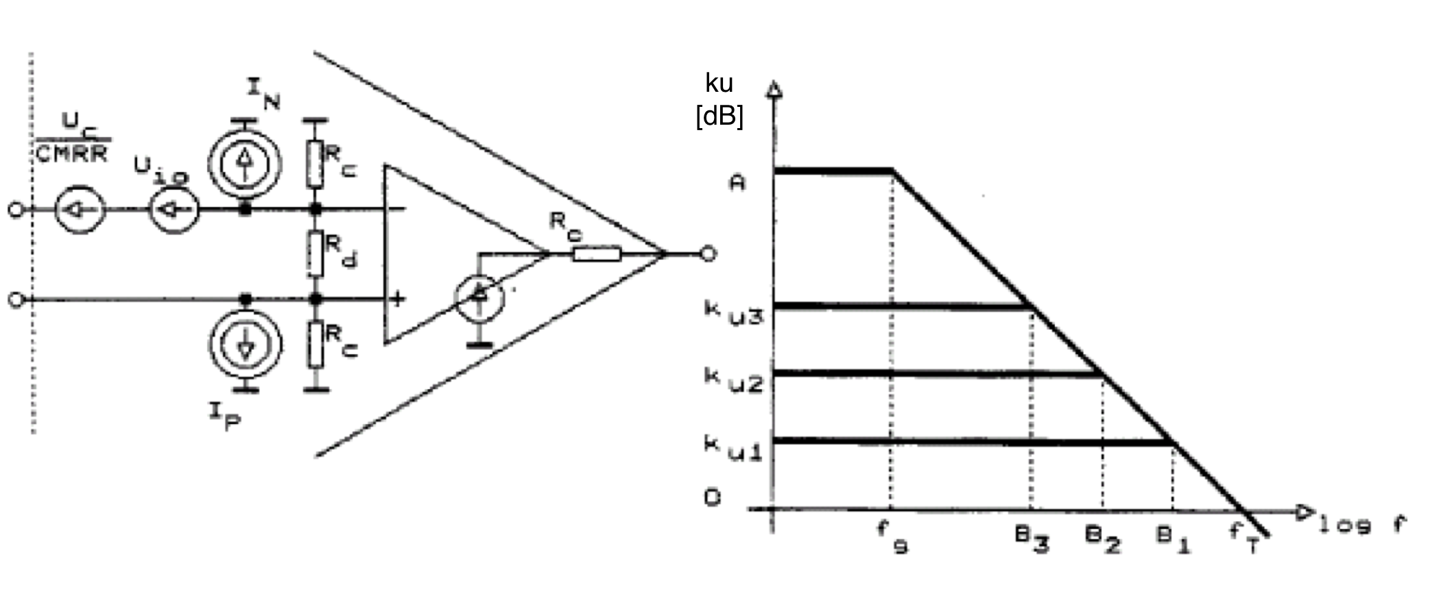
Figure 12 Figure 13