Basics of electronic ...

The aim of the exercise is to familiarize yourself with the basic applications of operational amplifiers and to learn about the properties of practically used electronic circuits with operational amplifiers.

Operational amplifiers can work with negative feedback loops containing not only resistors \(R_1\), \(R_2\), but also other elements taking their place in the circuit. If they are inductors or capacitors, the system is usually linear (applications: integrators, derivatives, filters of various types, etc.). On the other hand, if the elements of negative feedback circuits are diodes or transistors, the system is usually non-linear (applications: logarithm amplifiers, exponent amplifiers, etc.). In this exercise, only some applications of operational amplifiers in linear circuits will be considered. Frequency characteristics will most often be presented in the double-logarithmic coordinate system (log-log): on the ordinate axis, the voltage transfer function expressed in decibels, on the abscissa axis, the frequency in the logarithmic scale.

The voltage transmittance (defined as the quotient of the complex amplitudes \(k_u = \frac{U_2}{U_1}\) of the harmonic voltages) of the linear inverting amplifier (Fig. 1) is: \(k_u =−\frac{Z_2}{Z_1}\) assuming that the op-amp is ideal and has an open-loop gain \(A\) infinitely large, and \(Z_2\), \(Z_1\) are the impedances of the two-terminal components indicated in the figure (power supply is not shown in the diagram) .

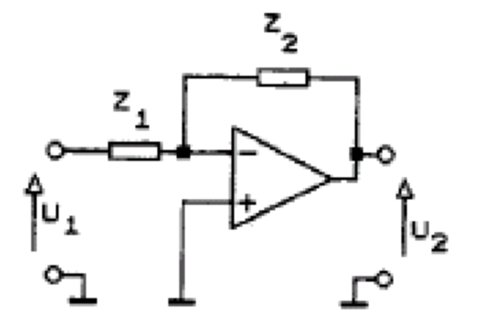
Figure 1

If \(Z_1 = R_1\) , \(Z_2 = R_2\) , then the circuit is an amplifier with gain \(k_u = −\frac{R_2}{R_1}\) , whose output voltage is proportional to the input voltage over the entire frequency range of the amplifier, i.e. from direct current to the upper limit frequency (Fig. 2), because here \( |k_u| \) does not depend on the frequency.

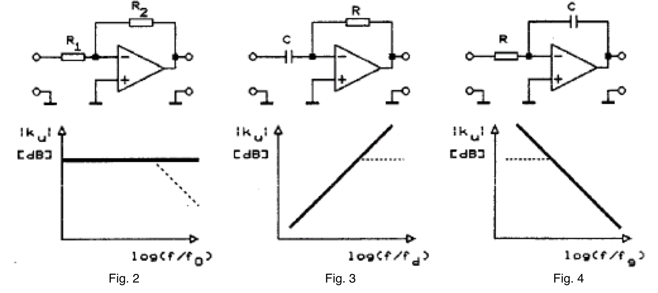
If \(Z_1 = \frac{1}{j\omega C} \), \(Z_2 = R\), then the circuit shown in Fig. 3 is characterized by the voltage transfer function \(k_u = −j\omega RC\), whose modulus \( |k_u| = \omega RC\) increases in proportion to the frequency. As we shall see later, the same circuit described in a different way, namely in the time domain rather than in the frequency domain, behaves under certain conditions as an input voltage differentiator.

If \(Z_1 = R\), \(Z_2 = \frac{1}{j\omega C}\), then the circuit shown in Fig. 4 is obtained whose voltage transfer function \(k_u=−\frac{1}{j \omega RC}\), and the modulus \( |k_u| = \frac{1}{\omega RC}\) decreases inversely proportional to the frequency. In the coordinate system adopted in Fig. 4 \(|k_u|\) is expressed in decibels, and the frequency scale is logarithmic, and then this relationship has the form of the straight line shown there. It can be shown that the same system described in the time domain behaves under certain conditions as a system that integrates the input voltage.

As \(Z_1\) and \(Z_2\) it is also possible to use passive two-terminal components composed of two or more R and C elements, because in practice inductive elements are not used due to their large dimensions and mass.

If \(Z_1 = R_1\), and as \(Z_2\), use a two-terminal component consisting of a resistor \(R_2\) and a capacitor with a capacitance \(C\) connected in parallel (Fig. 5), so that its resultant impedance \(Z_2 = \frac{R_2}{1+j\omega R_2 C}\), then the voltage transfer function of the entire system has the form of a single pole function:

\( ku = - \frac{R_2}{R_1 (1+j \omega R_2 C)} \);

the pole occurs for \( \omega_g=\frac{1}{R_2 C} \). Such a system can be said to be a low-pass filter with an upper cut-off frequency \(f_g=\frac{\omega_g}{2\pi}\), because, as it results from the presented frequency characteristics, it faithfully transfers harmonic signals with frequencies lower than \(f_g\), and attenuates signals with frequencies higher than \(f_g\); in other words, in the range \(f << f_g\) it works like the system in Fig.2, and in the range \(f>>f_g\) it works like the system in Fig.4.

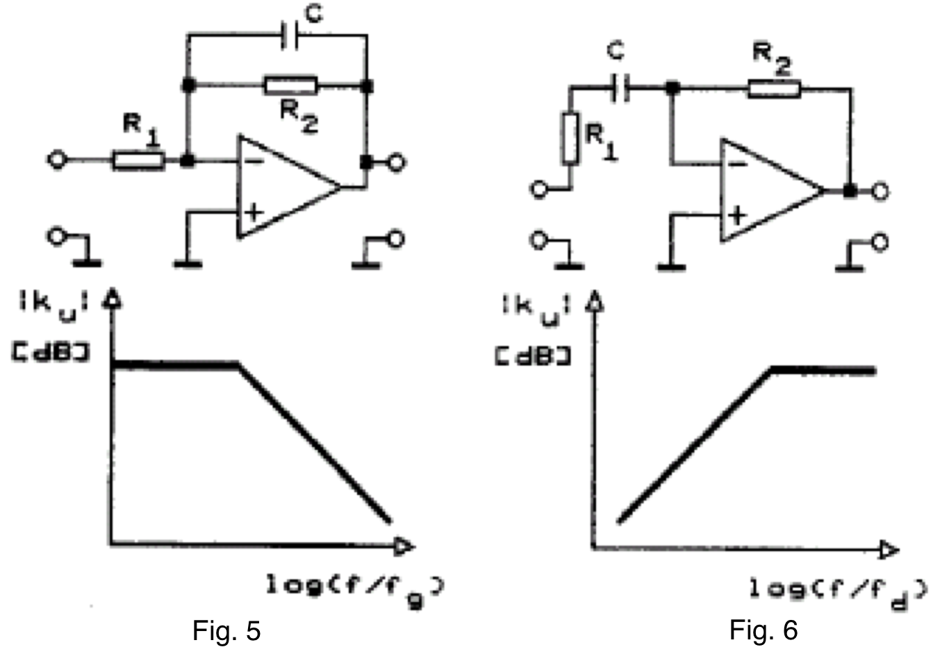
In the case of the system in Fig. 6, \(Z_1 = R_1+\frac{1}{j\omega C}\), \(Z_2 = R_2\) and the voltage transfer function of the system \(k_u = −\frac{j\omega R_2 C}{1+j\omega R_1 C}\), depends on the frequency in such a way that its modulus increases proportionally to the frequency in the range \(\omega<< \omega_d\) (similar to the system in Fig.3) , and does not depend on the frequency for \(\omega>> \omega_d\) . The frequency corresponding to \( \omega_d = \frac{1}{R_1 C}\) is the lower cut-off frequency of the circuit, which acts as a high-pass filter.

The last two systems are practical versions of the integrating (fig. 5) and differentiating (fig. 6) systems, respectively. Note here that in the log-log coordinate system, the characteristics of the ideal differentiator (fig.3) and integrator (fig.4) systems are straight lines with an angle of +20 dB/dec or -20 dB/dec. On the other hand, the practical systems in Fig. 5 or Fig. 6 are distinguished by the fact that in those frequency ranges in which these systems do not perform their basic tasks, i.e. integration or differentiation of signals, their amplification is limited: the corresponding sections of the characteristics are horizontal. This is dictated by the need to ensure stable operation of the differentiator system or to reduce the influence of drifts and disturbances on the operation of the integrator.